

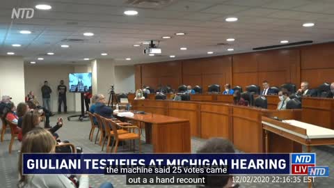
Dominion CEO vs Forensic Audit: somebody's lying
Dominion CEO testimony before Michigan panel concerning Antium county and Dominion voting Systems and the forensic audit thereof. Alternate evidence is overlaid in response to the CEO's claims.
447
views
11
comments

Dominion CEO testifies: wins record for most lies in 27 minutes (pretty sure)
Dominion CEO testifies to Michigan House on 15 Dec 2020 following forensic analysis of fraud in Antrim County
4
views
Riemann Sum with 2 Variables
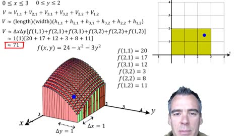
We approximate the volume under f(x,y) over the region where 0≤x≤3 and 0≤y≤2.
The volume is approximated in a Riemann Sum of 6 rectangular prisms and visualized in calcplot3D.
The process of taking a difficult problem and cutting it up into smaller easier problems is also discussed, as we find the volume of this solid by cutting it up into 6 rectangular columns. The underestimate is discussed. Each of the six volumes are calculated by find the length, width and height of each prism. The volumes are then summed and the graphic and approximated volume are concurrently shown in CalcPlot3D.
Finally, the next video is introduced within the context of finding a more accurate volume of the solid.
The link to the calcplot3D visualization is here:
https://c3d.libretexts.org/CalcPlot3D/index.html?type=region;region=x;visible=true;alpha=150;view=0;top2d=2;bot2d=0;umin=0;umax=3;top3d=24-x^2-3y^2;bot3d=0;grid=25,25;showriemann=true;xnum=3;ynum=2;partition=Inner;heightpt=4;showpts=false;mode=rect;polarform=t;polartop=2;polarbottom=0;polarmin=%CF%80/4;polarmax=3%CF%80/4&type=window;hsrmode=0;nomidpts=true;anaglyph=-1;center=8.479206834744925,4.8370832491824665,2.169257267842504,1;focus=0,0,0,1;up=-0.250790730365395,-0.20113018118593123,0.9469163953480297,1;transparent=false;alpha=140;twoviews=false;unlinkviews=false;axisextension=0.7;xaxislabel=x;yaxislabel=y;zaxislabel=z;edgeson=true;faceson=true;showbox=false;showaxes=true;showticks=true;perspective=true;centerxpercent=0.39645639607941685;centerypercent=0.5526315789473687;rotationsteps=30;autospin=true;xygrid=false;yzgrid=false;xzgrid=false;gridsonbox=false;gridplanes=false;gridcolor=rgb(128,128,128);xmin=-1;xmax=4;ymin=-1;ymax=4;zmin=-1;zmax=5;xscale=1;yscale=1;zscale=1;zcmin=-4;zcmax=4;zoom=0.627556;xscalefactor=1;yscalefactor=1;zscalefactor=0.1
48
views
How to find work done by 3D force field on object in motion
In this video I tackle a seemingly difficult math problem involving vector fields and space curves with a surprisingly easy method using a line integral.
Here’s the problem statement:
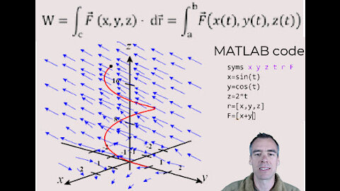
Compute the work done by the force field F ⃗(x,y,z)=(x+y) i ̂+(x-z) j ̂+(y+z) k ̂ on a mathematical bug walking along the helix parameterized by r ⃗(t)=〈sin(t),cos(t),2t〉 for 0≤t≤3π.
Ok if this seems rather involved well it is and this only becomes more clear if we take a look at this problem visually to get a handle on it, which you can pull up from the calcplot3d link below
You might imagine it’s rather hard problem to find the work done by this intricate force field on the bug over this convoluted path, but it’s actually pretty straightforward,
We can start off with the equation
And if we parameterize our x and y and z are functions of time, and our dr ⃗ translates into our velocity vector function, r ⃗ ‘(t)dt, and we’re integrating from time a to b.
Now this isn’t too bad, we already have our x, y and z defined above as part of r ⃗(t), and we’re given our a and b as our t range, so we actually have all we need at this point and can just plug into MATLAB
MATLAB
So in MATLAB first we’ll define our variables as usual
syms x y z t r F
then define the x,y and z values given with the provided definition of r ⃗(t)
x=sin(t)
y=cos(t)
z=2*t
then we can define our position function with these x,y and z values
r=[x,y,z]
And finally we can define the force field
F=[x+y,x-z,y+z]
And let’s go ahead and define our a and b limits for good measure
a=0
b=3*pi
Plugging this in we can find our work as the integral of the dot product of our force field F, with the derivative of our position function r wrt t, integrating wrt t for the limits t=a to t=b.
W=int(dot(F,diff(r,t)),t,[a,b])
That answers a bit ugly so we can convert to a decimal
double(ans)
and get ~196.5
And that’s it!
I finally take a look at the problem graphically again to make sure the work done by the force field on the bug is going to be positive, and that solves this seemingly difficult problem with some pretty quick mathematics and the help of MATLAB.
Calcplot3d link:
https://www.monroecc.edu/faculty/paulseeburger/calcnsf/CalcPlot3D/?type=vectorfield;vectorfield=vf;m=x+y;n=x-z;p=y+z;visible=true;scale=4;nx=5;ny=5;nz=5;mode=0;twod=false;constcol=true;color=rgb(0,0,255);norm=true;desystem=false&type=slider;slider=t;value=0;steps=30;pmin=0;pmax=10;repeat=true;bounce=false;waittime=1;careful=false;noanimate=false;name=-1&type=spacecurve;spacecurve=curve;x=sin(t);y=cos(t);z=2t;visible=true;tmin=0;tmax=3pi;tsteps=150;color=rgb(255,0,0);showtrace=true;tval=9.42477796076938;constcol=true;twod=false;arrows=;showpt=true;trace=false;vel=false;acc=false;osc=false;k=false;repeat=false;bounce=false;dashed=false;tanline=false;showtvector=false;shownvector=false;showbvector=false;showtnbeqs=false;showtnblabels=false;showoscplane=false;showrectplane=false;shownormplane=false&type=window;hsrmode=3;nomidpts=true;anaglyph=-1;center=7.067727288212191,6.363810234300481,3.0901699437493804,1;focus=0,0,0,1;up=-0.15450849718749132,-0.13912007574599797,0.9781476007338006,1;transparent=false;alpha=140;twoviews=false;unlinkviews=false;axisextension=0.7;xaxislabel=x;yaxislabel=y;zaxislabel=z;edgeson=true;faceson=true;showbox=false;showaxes=true;showticks=true;perspective=true;centerxpercent=0.5;centerypercent=0.5;rotationsteps=30;autospin=true;xygrid=false;yzgrid=false;xzgrid=false;gridsonbox=true;gridplanes=true;gridcolor=rgb(128,128,128);xmin=-2;xmax=2;ymin=-2;ymax=2;zmin=0;zmax=20;xscale=1;yscale=1;zscale=8;zcmin=0;zcmax=20;zoom=0.5496;xscalefactor=1;yscalefactor=1;zscalefactor=0.2
60
views
Introducing the Double Integral: Finding Volume Under Surface
Having looked at a Riemann Sum for approximating a volume in the last video, we now see how to transition this into an infinite Riemann Sum and finally into an integral, just as you may recall doing in integral calculus.
Suppose we wanted to find the area under our function f(x) between the points a is less than x is less than b. We break this up into m rectangles and sum up their areas to approximate the area under the curve, where Δx=(b-a)/m
and f(x_i ) was the height for each rectangle. And to find the exact area, we added up an infinite number of infinitesimally thin rectangles, and this infinite sum turned out to be the very definition of the integral.
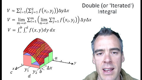
Now in 3-space, suppose we have a surface f(x,y)=24-x^2-y^2/3 and we wanted to find it’s volume between 0 is less than x is less than 3 and 0 is less than y is less than 2.
As in the previous video, we can estimate this volume by summing up some rectangular columns, each column of width and length Δx and Δy. We can formally define the widths as Δx=(b-a)/m=(3-0)/3=1 where a and b would be the lower and upper x limits of 0 and 3 and each has a height of the surface value at the corresponding x and y coordinates. So the volume of each rectangular column is ΔxΔy f(x_i,y_j). More generally we can call that ΔxΔy=ΔA for the area of each of chunk where i is like the i values in our integral calculus example, and j is our index for y.
Now we can add up these rectangular solids like we did in the previous video, but we’ll use summation notation this time to find our approximate volume. We'll use a summation nested within another summation because we are adding the heights for each of the 2 y increments, and doing that 3 times for each of the x increments, for what amounts to a total of 6 rectangular columns.
Now comes the fun part, we can find the exact volume by summing up an infinite number of rectangular columns that are infinitesimally thin in the x and y directions.
To do that me make some modifications to our prior equation by replacing our 3 increments in the x direction and 2 increments in the y direction with variables m and n, respectively, and taking the limit of our summation as m and n both approach infinity. This gives us our exact volume, so again we have one summation nested inside another, but these are infinite summations now, and we know that infinite sums of this form are the very definition of integrals, so we could change the inside summation to an integral where we brought that dy to the inner integral
and we could change the outside summation to an integral as well:
So above is the general form of a double integral to find the exact volume of a solid in 3-space. But to go back and apply this the problem we did in the previous video, that c and d were our y limits of 0 and 2 in this case, and that a and b were our x limits of 0 and 3 in this case, and that f(x,y) was our function 24-x^2-3y^2 .
In the next video we’ll go ahead and evaluate this using some basic calc2 skills while simultaneously showing how to evaluate it in MATLAB.
3
views
Evaluating a Double Integral by Hand
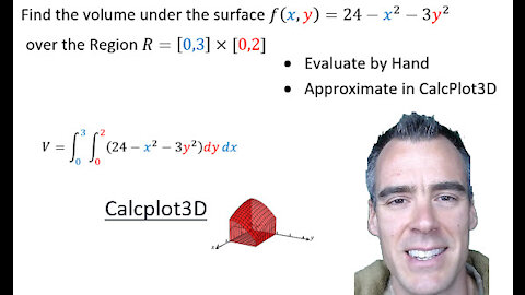
In the previous videos we looked at a Reimman sum for finding the volume of the function f(x)=24-x^2-3y^2 on the Region R=[0,3]×[0,2], which is a compact way of communicating the region where x is between 0 and 3 and y is between 0 and 2.
We then looked at translating that Reimman sum into an integral
Here we’ll quickly go through the nuts and bolts of evaluating this algebraically, comparing it to what we had in CP3D, and evaluating the integral with MATLAB.
The process is very similar to what you’re familiar with in calc 2, so let’s get started:
Basically, you just work from the inside out to get ‘partial’ integrals while treating one of the variables as a constant.
We will first evaluate the inside integral which is with respect to y,
So we add a y to the 24 constant, add a y to x^2 which we treat as a constant, and use the inverse power rule to integrate 3y^2
Next of course we evaluate by plugging in 2 and 0 for y
V=∫_0^3▒[24(2)-x^2 (2)-(2)^3 ]dx
Now we’ve integrated the inner integral, and next we integrate the outer integral, which is with respect to x this time
So first we take the antiderivatives…
Then we plug in 3 and 0 for x
And performing those operations we arrive at our final answer
V=102
Next we'll verify this in Calcplot 3d and in the next video we'll evaluate in MATLAB anddemonstrate Fubini's theorem.
1
view
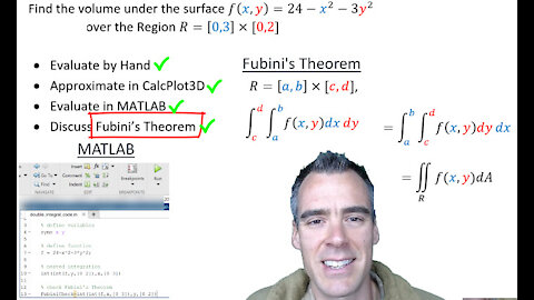
Evaluating a double integral and demonstrating Fubini's Theorem with MATLAB
In the last video we quickly go through the nuts and bolts of evaluating this algebraically, comparing it to what we had in CP3D, and here we'll evaluated the integral with MATLAB and use MATLAB to demonstrate Fubini's Theorem
First we define our x and y symbolic variables
syms x y
Then we define our function
f(x,y)=24-x^2-3*y^2;
And now we use the integrate command nested within another integrate command,
So our inner integral is wrt y between 0 and 2
And our outer integral is wrt x between 0 and 3
int(int(f,y,[0 2]),x,[0 3])
And there we have our answer of 23 confirmed
Finally, we can also compare this to our Reimann sum from CP3D
And if we go back to that and ratchet up our increments in the x and y directions we see that our Reimann sum gets pretty close to 102, further confirming our answer.
But one final question here, what if we switch around the order of integration, will that give us a different answer?
Well, I would encourage you to do just using the calculus steps above, but since hopefully you trust MATLAB now that we’ve confirmed our answer, let’s try it there..
And… we see this does in fact give us the same answer,
This illustrates ‘Fubini’s Theorem’
So we can freely switch our order of integration as long as we keep the bounds consistent and as long as those bounds are just numbers. In the next video, we’ll discuss what happens when those bounds are actually functions rather than numbers, but until then, take care
8
views
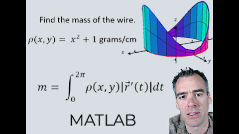
Example Problem: finding the mass of a wire with a scalar line integral
Example Problem: finding the mass of a wire with a scalar line integral.
I set up the integral, evaluate it in MATLAB, and also take a look at it graphically.
Here is the problem statement:
Let W represent a thin wire bend in the shape of a circle of radius 3 centered at the origin in the xy-plane. The density of the wire is given by ρ(x,y)= x^2+1 grams/cm at every point (x,y) along the wire. Find the mass of the wire.
So we can start with our equation for the scalar line integral
We insert our density as the function where m is total mass we're looking for and we know that ds becomes |r ⃗^' (t)| dt.
But we're not sure exactly what to plug in for a or b or what |r ⃗^' (t)| is yet.
So to find those we graph it out.
We need to find parametric equations for the x and y values as a function of time .
This takes a little creativity but as you may recall unit circle can be defined by parametric functions of sine and cosine for our x and y
So if we defined
x=cos(t)
and
y=sin(t)
this would give us a unit circle starting at the point
(1,0)
at
t=0=a
and going all the way around the circle through
t=2π=b
so those t values will be our a and b.
Our circle is scaled up from that by 3, so we can just multiply each component by 3, yielding
x=3cos(t)
and
y=3sin(t)
so r would be
r ⃗(t)= 〈3cos(t), 3sin(t)〉
But we need
|r ⃗^' (t)|
This isn't too hard to figure out but let's let MATLAB take it from here. But first, let me note that there are infinite combinations of sin and cos parameterizations that would work for this. The parameterizations could start at different places and go different speeds, but as we are parameterized to take one loop around the circle, we’ll get the same correct answer.
But let’s go with what we’ve got here and plug it into MATLAB
And start of by defining all the symbolic variables and let’s just define everything
syms x y r t rho
Then we can define the x we found
x=3*cos(t)
And the y we found
y=3*sin(t)
And combine those together for r
r=[x,y]
and we can also define rho as
rho=x^2+1
And finally plug those into our integral of our rho function x^2+1 times the magnitude of the derivative of r (and this is a common place to miss something) by using the norm and diff commands, wrt t, wrt t from t = 0 to 2pi
m=int(rho*norm(diff(r,t)),t,[0,2*pi])
This yields a tidy value of
33π
which is our final answer but let's do one last thing
I may be going too far with this but personally I need to understand things graphically so let's imagine we have our circle here in 3 space.
Now let's imagine our z axis corresponds to the density of our function, so at each of these point along our red circle we have a height over it in blue corresponding to how dense the wire is at that point.
Then that line integral we found, which was the total mass of the wire, corresponds graphically here to the area underneath this blue line,
So our line integral is still the area under a curve, It's just that in this case the height of that curve has the physical meaning of density.
So I hope this idea of a line integral is making sense to you, and we'll move on from here to take a look at line integrals over vector fields next.
21
views

Rand Paul and Judge Starr to US Senate: 60 election court cases decided on procedural issues, not merit
Rand Paul and Judge Starr address democratic 59-2 court case talking point in US Senate
157
views

Wisconsin Attorney James Troupis explains 200,000+ corrupted votes to US Senate
Wisconsin Attorney James Troupis explains 200,000+ corrupted votes to US Senate
141
views

Pennslyvania Rep Ryan summarizes PA case to US Senate
Pennslyvania Rep Ryan summarizes PA case to US Senate - '75,000 ballots added after 17 Nov'
97
views

Sidney Powell summarizes Georgia case, judge dismisses: "too late and I don't have authority'
Sidney Powell summarizes Georgia case, judge dismisses because "its too late and I don't have authority'
72
views
2
comments

Biden says 250,000 will die from COVID in Dec 2020
Biden says 250,000 will die from COVID in Dec 2020
66
views
Giulianni closes down MI hearings with gusto, authority and fireworks
Giulianni closes down MI hearings with gusto, authority and fireworks
20
views


Michigan pollworker Ms. Jacobs testifies of illegal process, drops supervisor names
Michigan pollworker Ms. Jacobs testifies of illegal process, drops supervisor names

Constitutional Scholar Dr. Eastman discusses options with Georgia legislature
Constitutional Scholar Dr. Eastman discusses options with Georgia legislature
1
view

Melissa Caronne strikes again and MI house hearings
Melissa Caronne strikes again and MI house hearings
8
views

Attorney who broke GA ballot fraud video (Jackie Pick) debunks the debunkers
Attorney who broke GA ballot fraud video (Jackie Pick) debunks the debunkers
8
views


Cybersecurity expert Col Wills discuss foreign interefence in 2020 election
Cybersecurity expert Col Wills discuss foreign interefence in 2020 election
2
views


Garland Favorito gives update on Dominion switching 37 votes in Ware County
Garland Favorito gives update on Dominion switching 37 votes in Ware County
8
views


Senator Colbeck testifies at Michigan Senate Hearing on Election Issues
Senator Colbeck testifies at Michigan Senate Hearing on Election Issues
1
view