Euler's Method for Solving Differential Equations Explained, Example - Calculus
Euler's method is a simple numerical technique for approximating solutions to first-order ordinary differential equations (ODEs) with an initial value. It works by iteratively moving along the tangent line at each step, using the derivative to find the slope, and advancing the solution by a small step size ('h') to estimate the next point on the solution curve. The basic formula is y₁ = y₀ + h * f(x₀, y₀), where y₀ is the initial value, x₀ is the initial x-value, h is the step size, and f(x₀, y₀) is the slope at the starting point derived from the differential equation.
💡How it Works
• Problem Setup: You start with a differential equation in the form y' = f(x, y) and an initial condition (x₀, y₀).
• Choose a Step Size (h): This is the small increment you'll use to move from one point to the next along the x-axis.
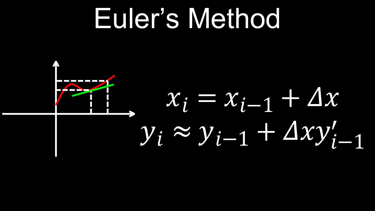
• Calculate the Slope: At the current point (xₙ, yₙ), find the slope using the differential equation: m = f(xₙ, yₙ).
• Estimate the Next Point: Move from the current point by taking a small step of size 'h' along the tangent line. The new y-value is calculated as: yₙ₊₁ = yₙ + h * f(xₙ, yₙ).
• Repeat: Use the new point (xₙ₊₁, yₙ₊₁) as your starting point for the next step and repeat the process to find the next approximation.
💡Key Formula
The core of Euler's method is the iterative formula:
• **yₙ₊₁ = yₙ + h
• f(xₙ, yₙ)**
💡Example Application
Imagine you want to find the approximate value of a solution to y' = 2x and y(1) = 3, using a step size of h = 0.1.
• Initial Condition: (x₀, y₀) = (1, 3).
• Step 1:
⚬ Calculate f(x₀, y₀) = f(1, 3) = 2 * 1 = 2.
⚬ Calculate y₁ = y₀ + h * f(x₀, y₀) = 3 + 0.1 * 2 = 3.2.
• Step 2:
⚬ The new point is (x₁, y₁) = (1 + 0.1, 3.2) = (1.1, 3.2).
⚬ Calculate f(x₁, y₁) = f(1.1, 3.2) = 2 * 1.1 = 2.2.
⚬ Calculate y₂ = y₁ + h * f(x₁, y₁) = 3.2 + 0.1 * 2.2 = 3.42.
You continue this process to find subsequent points.
💡Accuracy and Limitations
• Step Size (h): The accuracy of Euler's method depends on the step size. Smaller step sizes generally lead to better approximations but require more computational steps.
• First-Order Method: It is a first-order method, meaning it assumes the slope remains constant over the small interval, which introduces some error.
• Applications: Despite its limitations, Euler's method is fundamental in computational science and forms the basis for more complex numerical methods used to solve and simulate differential equations in fields like engineering and physics.
💡Worksheets are provided in PDF format to further improve your understanding:
• Questions Worksheet: https://drive.google.com/file/d/1DMK4EA0f8SfF4SgdiOZ39F73He_YWIwe/view?usp=drive_link
• Answers: https://drive.google.com/file/d/1QpzjiCPjfoxydzZqvjyJJsqv9jyRLZ0o/view?usp=drive_link
💡Chapters:
00:00 Euler's method
01:23 Worked example
🔔Don’t forget to Like, Share & Subscribe for more easy-to-follow Calculus tutorials.
🔔Subscribe: https://rumble.com/user/drofeng
_______________________
⏩Playlist Link: https://rumble.com/playlists/Ptm8YeEDb_g
_______________________
💥 Follow us on Social Media 💥
🎵TikTok: https://www.tiktok.com/@drofeng?lang=en
𝕏: https://x.com/DrOfEng
🥊: https://youtube.com/@drofeng
-
 UPCOMING
Caleb Hammer
2 hours agoThe Most Hated Person In Financial Audit History
621 -
 UPCOMING
The Big Mig™
2 hours agoTraitors Committing Sedition Says President Trump
1654 -
 30:49
30:49
MetatronHistory
16 hours agoThe Truth about Women Warriors Based on Facts, Evidence and Sources
5K3 -
 15:17
15:17
IsaacButterfield
6 hours ago $0.44 earnedAustralia’s Most Hated Politician
4.62K3 -
 4:28
4:28
MudandMunitions
12 hours agoSHOT Show 2026 Is Locked In and I’m a Gundie Nominee!
3.27K -
 1:19:44
Chad Prather
19 hours agoWhen God Shakes the Room: Bold Faith in a Fearful World
62.4K44 -
 58:40
58:40
Julie Green Ministries
4 hours agoLIVE WITH JULIE
85.1K143 -
 1:01:10
Crypto Power Hour
12 hours ago $3.02 earnedAnimus Bitcoin Technology
29.2K8 -
 2:22:18
Game On!
19 hours ago $3.32 earnedAnother FOOTBALL FRIDAY! Weekend Preview And BEST BETS!
24.6K1 -
 31:55
31:55
ZeeeMedia
20 hours agoHow Gold & Silver Fight Against Digital ID ft. Bill Armour | Daily Pulse Ep 148
23.3K10