Microsoft Excel Midterm Exam - September 2025 - Embedded with MOS Microsoft Excel (54 questions)

Microsoft Excel Midterm Exam – September 2025 (Time: 75 minutes)
Question 1: Write your first name and last name on cell B4 and C4. Change the theme is Office.
Question 2: Create the formula with the function to make the full name by your first name and last name on cell D4. Apply the horizontal alignent of full name with Left (Indent). Set the indent to 1.
Question 3: Edit the name on cell C5 from “John” into “Jackson”.
Question 4: In column A, using the Autofill for ID number.
Question 5: Create the format of the email firstname.lastname@abc.com (For example: John Jack will be john.jack@abc.com ) and then apply flash fill.
Question 6: Remove the hyperlink of all email address, except your email. In this one, we need to edit your hyperlink with ScreenTip: I am examinee.
Question 7: Drag and fill the value from cell G3 to J3 so they can show all the months. Similar with the G17 to J17.
Question 8: Adjust the column from A to M to see all the information.
Question 9: Create the formula with the function to count all students in the table on cell U3 by First Name.
Question 10: Adjust the row 1 into 25.00 points.
Question 11: Apply merge and center of the headline from A1 to M1.
Question 12: Apply the cell style for the heading – 40% - Accent 3 and change the font into Algerian with 20 points. Edit the “Scholarshop” into “Scholarship”.
Question 13: Delete the row 14.
Question 14: Apply Italic and Bold font for cell B14. Change the font to 12 points and Times New Roman.
Question 15: Hide the row 14 because we do not want to show the person who approved the list.
Question 16: Insert a new row in row 2 and apply clear the format for A2:M2.
Question 17: Write the subtitle on B2 with Sep 23,2025 and apply merge and center for A2:M2. Then, apply the cell style Heading 2. Later, change the font into 24 points.
Question 18: Remane in cell F4 with Grants instead of Money.
Question 19: Format the table from A4:M11 with Dark Green, Table Style Medium 4.
Question 20: Change the column width on column M with 10 and then apply the wrap text for cell M3.
Question 21: Create the formula with function to find the total scholarship that distribute from September to December.
Question 22: Create the formula without the function to calculate the total funds that we need to distribute next year from the grants in the column L. After that, apply the Accounting format with no decimal place for F5:L11.
Question 23: Create the formula with the function to show that if the fund is greater than 0, it will show Yes. If not, it will show No in the column M.
Question 24: Insert a new row inside the table between “Distribute next year?” and “Remaining funds” for the table with the title “Trend” on M4. Insert the sparklines in M5 for the values from September to December. Change the style of sparklines with Green, Sparkline Style Accent 3, Lighter 40%. The sparklines have orange high point and purple low point.
Question 24: Using the conditional formatting for value in F5:F11 to find which grant is more than $2000 with Green Fill with Dark Red Text.
Question 25: Create the formula with the function to calculate the total funds in G18 and copy the formula for the rest.
Question 26: Create the formula with the function to calculate the average funds in G19 and copy the formula for the rest.
Question 27: Create the formula with the function to calculate the maximum funds in G20 and copy the formula for the rest.
Question 28: Create the formula with the function to calculate the minimum funds in G21 and copy the formula for the rest.
Question 29: Create the formula without the function to calculate the range funds in G22 from maximum and minimum value. Then we copy the formula for the rest. Finally, apply Accounting number format for G18:K22 with no decimal place.
Question 30: Format the table from F17:K22. We need to apply the All Border with the border color is Green. The title of the month will be Bold with White, Background 1 font color. Moreover, Fill color of the title is Dark Teal, Accent 1.
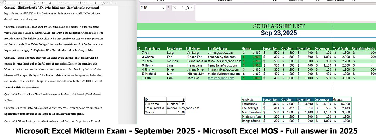
Question 31: Highlight the table A4:N11 with defined name: List of scholarship students and hightlight the table F17:K22 with defined name: Analysis. About the table B17:C20, using the defined name from Left column.
Question 32: Insert the pie chart about the total funds based on 4 months (Not the total grants) with the title name: Funds by months. Change the layout 2 and quick style 5. Change the color to monochromatic 1. Put the label on the chart so that they can show the category name, percentage and the show leader lines. Delete the legend because they repeat the month. After that, select the largest portion and apply Pie Explostion 10%. Move the chart below the Analysis Table.
Question 33: Insert the combo chart with the Grants by the line chart and 4 months with the clustered column chart based on the full name of each student. Deselect the secondary axis. Move the chart into the new worksheet with the sheet name is “Scholarship by the Name” with tab color is Blue. Apply the layout 5 for the chart. Make sure the number appear on the bar chart and line chart in Outside End. Change the maximum bounds for vertical axis to 4000. After that we need to Hide this Sheet Name.
Question 34: Return back the Sheet 1 and then rename the sheet by “Scholarship” and tab color is Green.
Question 35: Sort the List of scholarship students in two levels. We need to sort the full name in alphabetical order then based on the largest to the smallest value of the grants.
Question 36: We need to inspect workbook and remove all Document Properties and Personal Information.
Question 37: In range B17:C20, create the formula with the function to find the information of student ID number 5 and fill all the table based on the information on the left side.
Question 38: We need to add developer in the ribbon. We need to record the macro so we can insert the new column from “List of scholarship students” defined name because we will have new students in the future. After finishing the record the macro, undo the insert step. Add the button on cell P4 with “Add the row” on the button. Lastly, we need to assign the macro for this button.
Question 39: About the table in cell S3, create the formula with the function to count the numbers of students more than 2000$ in grants of scholarships, and the total of funds for students who have more than 2000$ in grants of scholarships in V5:V6. Merge and center of S4:T4, S5:T5 and S6:T6.
Question 40: We need to apply the advanced filter by make the criteria to find the students who have more than 2000$ in grants of scholarship. Copy the header from the table and put in cell A40. We put the same header from “List of scholarship students” and put the criteria with greater than 2000 below the header Grants. Then insert the result at A1 into the new worksheet with the name “Scholarship over $2000” with the tab color Orange. Then we apply Move and Copy at the end with the second worksheet with the name “Scholarship next year” and clear all the content except the header for future usage. Protect the second worksheet with password “abc123” and accept the default selections.
Question 41: In the table at range S17:Y24, it is the list of teachers who approved the scholarship. We need to use first 3 letter for the teacher code in cell U18 and put these codes in All capital letter. Fill the rest the information.
Question 42: Create the formula with the function to show True or False in cell W17 if the teacher is from Business Administration and Gender is Male. Fill the rest the information.
Question 43: Create the formula with the function to show True or False in cell X17 if the teacher is from Finance or Gender is Female. Fill the rest the information.
Question 44: Create the PivotTable from table S17:Y24 to new worksheet and drag this worksheet next to “Scholarship” with a new name “Teachers”.
Question 45: In new worksheet “Teachers”. Edit the row labels is Major and drag the Major in Row heading. Edit the column labels is Gender and drag the Gender in Column heading. About the values, we need to find the average of Fund Sponsorships by Gender. Rename the Grand Total into Average Funds. Change the number into Currency format with two decimal places. Change the format of PivotTable into Outline Form. Put Teacher code into filter for future using.
Question 46: Add the slicer based on Major. We need only show the table based on Accounting and Finance.
Question 47: Return back the Scholarship worksheet. Go to table S27:X33. Write 2% at cell S27 and use that for the data table with Row input cell. Format value in S27 as the percentage and the result as the accounting and both of them are zero decimal place.
Question 48: Go to the right. There are 2 scenario to raise the funds. In scenario 1, we need to find the total number of people to raise the funds up to $1000 with the average can give $10. In scenario 2, we need to find the total package 1 and package 2 so that we can get the maximum funds for the scholarship. Save and load these result in new worksheet with default name for scenario 2. Show all the formula on the right side of Scenario 2 and answer the selection of scenario by the function.
Question 49: Add the comment in the cell S35 with the comment “I had done the exam!”, including the exclaimation mark. In the cell S36, using the format with the function to show the date that you edit the file. In the cell S37, using the format with the function to show the weekday from S36.
Question 50: Change the Orientation in Landscape. Hide the gridlines and headings
Question 51: Change the Margin with Top and Bottom by 1 point. Center the page horizontally.
Question 52: Custom the footer. On the left section, put your full name. On the center section, insert the file name. On the right section, insert the sheet name.
Question 53: Create a new worksheet to link all visible worksheets by cell A1 (except hidden and protected sheet) with the name of these worksheets in one place and drag this worksheet at the beginning of the document.
Question 54: Save the new file name with Full Name next to the title of this file. For example, full name is John Jack so the file is JohnJack Midterm Exam Microsoft Excel.
THE END