New Perspectives Excel 365/2021 | Modules 1-4: SAM Capstone Project 1b| Saxon Municipal Government

Saxon Municipal Government
FORMATTING, FORMULAS, AND CHARTS
GETTING STARTED


Save the file NP_EX365_2021_CS1-4b_FirstLastName_1.xlsx as
NP_EX365_2021_CS1-4b_FirstLastName_2.xlsx
o
o
Edit the file name by changing “1” to “2”.
If you do not see the .xlsx file extension, do not type it. The file
extension will be added for you automatically.
With the file NP_EX365_2021_CS1-4b_FirstLastName_2.xlsx open, ensure
that your first and last name is displayed in cell B6 of the Documentation
worksheet.
o
If cell B6 does not display your name, delete the file and download a new
copy.
PROJECT STEPS
1.
2.
3.
4.
5.
6.
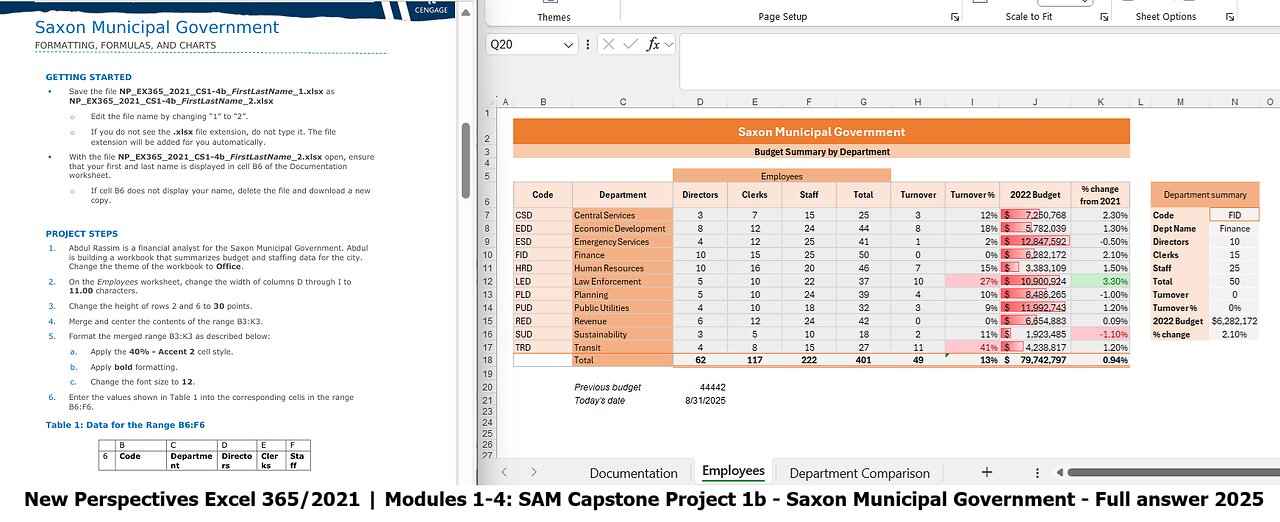
Abdul Rassim is a financial analyst for the Saxon Municipal Government. Abdul
is building a workbook that summarizes budget and staffing data for the city.
Change the theme of the workbook to Office.
On the Employees worksheet, change the width of columns D through I to
11.00 characters.
Change the height of rows 2 and 6 to 30 points.
Merge and center the contents of the range B3:K3.
Format the merged range B3:K3 as described below:
a.
b.
c.
Apply the 40% - Accent 2 cell style.
Apply bold formatting.
Change the font size to 12.
Enter the values shown in Table 1 into the corresponding cells in the range
B6:F6.
Table 1: Data for the Range B6:F6
B
C
D
E
F
6 Code
Departme
nt
Directo
rs
Cler
ks
Sta
f
7.

19. In the Bottom Five Depts - 2022 2-D pie chart (located in the range J19:P38),
make the following changes:
a.
b.
Change the data labels to display only the percentage and a label position
of Inside End.
Reposition the legend on the right side of the chart.
20. Update the Top Five Departments column chart in the range B19:H39 as
follows:
a.
b.
c.
Change the maximum bound of the left vertical axis to 13,000,000.
Add axis titles to the chart. Use Budgeted $ as the left vertical title, use
Total Budget as the right vertical title, and remove the horizontal axis
title.
Apply a shape fill to the plot area using the Gray, Accent 3, Lighter
80% fill color.
21. Delete the Projections worksheet.
8.
9.
Format the range B6:K6 as described below:
a.
b.
c.
d.
Center cell contents.
Change the font size to 11 point.
Change the background color to Orange, Accent 2, Lighter 80% (6th
column, 2nd row on the Theme Colors palette).
Apply Wrap Text to the text in cell K6.
Select the range B7:K17 and then add a Light Gray, Background 2, Darker
10% (2nd row, 3rd column in the Theme Colors palette) border to all sides of
each cell.
Select the range B18:K18 and then add a thin top border to each cell using
Orange, Accent 2 (1st row, 6th column in the Theme Colors palette).
10. Select the range I7:I17 and then format the range as described below:
a.
b.
Format the range with the Percentage number format with zero decimal
places.
Add a Highlight Cells conditional formatting rule that formats cells that
are greater than 20% as Light Red Fill with Dark Red Text.
11. Select the range J7:J17 and then use conditional formatting to add gradient fill
red data bars.
12. Select the range K7:K17 and then add top/bottom conditional formatting rules
to format the top 5% of values as Green Fill with Dark Green Text and the
bottom 5% of values as Light Red Fill with Dark Red Text.
13. Enter a formula in cell N8 using the VLOOKUP function to find an exact match
for the department code. Look up the department code (cell N7) using an
absolute reference, search the employee table data (the range B7:K17) using
absolute references, and return the department name (the 2nd column).
14. Copy the formula in cell N8 to the range N9:N16, pasting the formula only, and
then edit the copied formulas to return the value from the column indicated by
the label in column M.
15. In cell D21, enter a formula using the TODAY function that displays the current
date.
16. Delete column P.
17. Hide row 22.
18. On the Department Comparison worksheet, create a 2-D pie chart based on the
non-adjacent range B12:B16 and F12:F16. Modify the chart as described
below:
a.
b.
c.
Resize and reposition the chart so that the upper-left corner is located
within cell J4 and the lower-right corner is located within cell P17.
Apply Chart Style 4 to the chart.
Enter Bottom Five Depts - 2025 as the chart title

#MicrosoftExcel
#Microsoft
#MicrosoftOffice
#NewPerspectives
#NewPerspectivesExcel
#SAMProject
#SAMCapstone