Independent Project 7-6 - Excel Project - The Hamilton Civic Center (Full answer in 2025)

Independent Project 7-6
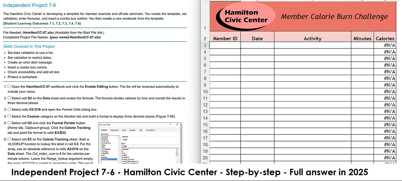
The Hamilton Civic Center is developing a template for member exercise and off-site seminars. You create the template, set
validation, enter formulas, and insert a combo box control. You then create a new workbook from the template.
[Student Learning Outcomes 7.1, 7.2, 7.3, 7.4, 7.6]
File Needed: HamiltonCC-07.xlsx (Available from the Start File link.)
Completed Project File Names: [your name]-HamiltonCC-07.xlsx
Skills Covered in This Project
Set data validation to use a list.
Set validation to restrict dates.
Create an error alert message.
Insert a combo box control.
Check accessibility and add alt text.
Protect a worksheet.
1.
2.
3.
4.
5.
6.
7.
8.
9.
Open the HamiltonCC-07 workbook and click the Enable Editing button. The file will be renamed automatically to
include your name.
Select cell D2 on the Data sheet and review the formula. The formula divides calories by time and rounds the results to
three decimal places.
Select cells D2:D10 and open the Format Cells dialog box.
Select the Custom category on the Number tab and build a format to display three decimal places (Figure 7-69).
Select cell D2 and click the Format Painter button
[Home tab, Clipboard group]. Click the Calorie Tracking
tab and paint the format to cells E3:E33.
Select cell E3 on the Calorie Tracking sheet. Start a
VLOOKUP function to lookup the label in cell C3. For the
array, use an absolute reference to cells A2:D10 on the
Data sheet. The Col_index_num is 4 for the calories per
minute column. Leave the Range_lookup argument empty;
the array (A2:D10) is sorted in ascending order. The result
of the VLOOKUP formula is calories per minute for the
exercise (Figure 7-70).
Edit the formula in cell E3 to multiply the results by the
number of minutes in cell D3.
Copy the formula in cell E3 to cells E4:E33. The #N/A
error message displays in rows where no data displays.
Figure 7-69 Custom format for values
Select cells C3:C33 and set data validation to use the list
of activity names on the Data sheet. Do not use an input message or an error alert.
10. Select the Calorie Tracking sheet and delete the data in cells A3:D23.
1/3
https://elearn.jscc.edu/d2l/le/content/8430010/viewContent/69587087/View
4/8/2021
SIMnet - Excel 2019 In Practice - Ch 7 Independent Project 7-6
11.
12.
13.
14.
15.
16.
Select cells B3:B33 and set data validation to use a
Date that is less than or equal to TODAY (Figure 7-71).
Include a Stop error alert with a title of Check Date and a
message of Date must be today or in the past. including
the period.
Select cells A3:D33 and remove the Locked cell
property. Select cell A3 to position the insertion point.
Display the Developer tab on the Ribbon and click the
Data worksheet tab.
Draw a combo box control to cover cell F8 and open its
Format Control dialog box. Select cells G8:G11 for the
Input range and type f8 in the Cell link box (Figure 7-72).
Figure 7-70 VLOOKUP formula
Deselect the control and then select Second from the control. The linked cell
is under the control and hidden from view.
Click the Hospital Seminars tab and select cell D4. This cell has Center
Across Selection alignment applied.
17. Select cell D4 and use CONCAT and INDEX to display the result from the
combo box, concatenating the Index results to the word “Quarter.”
a. Start a CONCAT function [Text group].
b.
c.
d.
Use the INDEX function with the first arguments list as the Text1
argument.
Choose cells G8:G11 on the Data sheet for the Array
argument and cell F8 for the Row_num argument. You
can select the combo box control or type f8 after the
sheet name (Figure 7-73). When the array is one
column, a Column_num argument is not necessary.
Click between the two ending parentheses in the
Formula bar to return to the CONCAT arguments and
type a comma (,) to move to the Text2 argument. (If you
accidentally click OK, click the Insert Function button to
re-open the Function Arguments dialog box.)
Figure 7-71 Data validation for dates
e.
f.
18.
Click the Text2 box, press Spacebar, type Quarter,
and click OK. (Figure 7-74).
Format cell D4 as bold italic 16 pt.
Select the Data sheet, select Third from the combo box
control, and return to the Hospital Seminars sheet to see
the results.
19.
20.
21.
22.
23.
24.
25.
26.
Select cell D4 and cells D6:G10 on the Hospital
Seminars sheet and remove the Locked property.
Delete the contents of cells D6:G10 and select cell D6.
Check accessibility and add the alternative text Hamilton
Civic Center Logo to both pictures in the workbook.
Select cell D6 on the Hospital Seminars sheet and cell
A3 on the Calorie Tracking sheet.
Protect the Hospital Seminars sheet and the Calorie
Tracking sheet, both without passwords.
Save and close the workbook (Figure 7-75).
Upload and save your project file.
Submit project for grading