Shelly Cashman Excel 2019 | Module 6: End of Module Project 1| Murray Medical (Update 2025)

Shelly Cashman Excel 2019 | Module 6: End of Module Project 1

Murray Medical
CREATE, SORT, AND QUERY TABLES

GETTING STARTED
• Open the file SC_EX19_EOM6-1_FirstLastName_1.xlsx, available for download from the SAM website.
• Save the file as SC_EX19_EOM6-1_FirstLastName_2.xlsx by changing the “1” to a “2”.
o If you do not see the .xlsx file extension in the Save As dialog box, do not type it. The program will add the file extension for you automatically.
• With the file SC_EX19_EOM6-1_FirstLastName_2.xlsx still open, ensure that your first and last name is displayed in cell B6 of the Documentation sheet.
o If cell B6 does not display your name, delete the file and download a new copy from the SAM website.
PROJECT STEPS
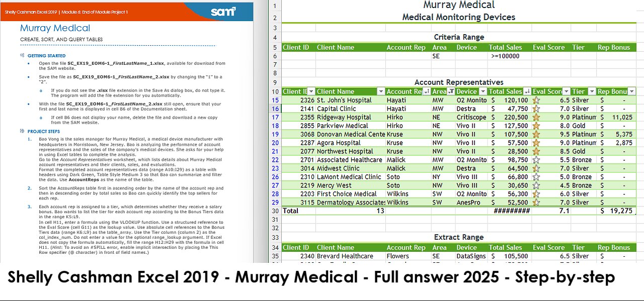
1. Bao Vong is the sales manager for Murray Medical, a medical device manufacturer with headquarters in Morristown, New Jersey. Bao is analyzing the performance of account representatives and the sales of the company's medical devices. She asks for your help in using Excel tables to complete the analysis.
Go to the Account Representatives worksheet, which lists details about Murray Medical account representatives and their clients, sales, and evaluations.
Format the completed account representatives data (range A10:I29) as a table with headers using Dark Green, Table Style Medium 3 so that Bao can summarize and filter the data. Use AccountReps as the name of the table.
2. Sort the AccountReps table first in ascending order by the name of the account rep and then in descending order by total sales so Bao can quickly identify the top sellers for each rep.
3. Each account rep is assigned to a tier, which determines whether they receive a salary bonus. Bao wants to list the tier for each account rep according to the Bonus Tiers data in the range K5:L9.
In cell H11, enter a formula using the VLOOKUP function. Use a structured reference to the Eval Score (cell G11) as the lookup value. Use absolute cell references to the Bonus Tiers data (range K6:L9) as the table_array. Use the Tier column (column 2) as the col_index_num. Do not enter a value for the optional range_lookup argument. If Excel does not copy the formula automatically, fill the range H12:H29 with the formula in cell H11. (Hint: To avoid an #SPILL error, enable implicit intersection by placing the This Row specifier (@ character) in front of field names.)

4. Murray Medical awards a bonus of 5% (.05) to account reps who earn Platinum-tier ratings from their clients. In cell I11, enter a formula using the IF function and structured references that tests whether the value in the Tier field is equal to "Platinum". If it is, multiply the value in the Total Sales field by 0.05. Otherwise, enter 0 (zero) in the cell. If Excel does not copy the formula automatically, fill the range I12:I29 with the formula in cell I11. (Hint: To avoid an #SPILL error, enable implicit intersection by placing the This Row specifier (@ character) in front of field names.)

5. Bao asks you to identify the account reps with high, average, and low evaluation scores. In the Eval Score column (range G11:G29), create a new Icon Set conditional formatting rule using the 3 Stars icons. Edit the rule to display a shaded star in cells with a Number type value greater than or equal to 8. Display a half-shaded star in cells with a Number type greater than or equal to 6. Display an unshaded star in cells with a Number type value less than 6.
6. Add a Total Row to the AccountReps table, which automatically totals the rep bonuses.
Using the total row, display the count of client names, the sum of the total sales, and the average of the eval scores.
7. In the range N6:O8, Bao wants to list key findings from the data in the AccountReps table. In cell O6, enter a formula using the DAVERAGE function to average the sales of the Destra medical device. Use a range reference to the AccountReps table (range A10:I29) as the database, "Total Sales" as the field, and the range Q5:Q6 as the criteria.
8. In cell O7, enter a formula using the SUMIF function that totals the sales for the Destra medical device. Use a range reference to the Device values (range E11:E29) as the range, cell Q6 as the criteria, and a range reference to the Total Sales values (range F11:F29) as the sum_range.
9. In cell O8, enter a formula using the COUNTIF function that counts the number of Destra devices, using a structured reference to the Device column (AccountReps[Device]) as the range and cell Q6 as the criteria.
10. Bao wants to identify clients in the southeast with total sales of $100,000 or more, and then list them in a separate part of the worksheet. In cell D6, enter a criterion to select clients in the SE Area. In cell F6, enter a criterion to select Total Sales greater than or equal to 100000. Create an advanced filter using the data in the AccountReps table (range A10:I29) as the List range. Use the range A5:I6 as the Criteria range. Copy the results to another location, starting in the range A34:I34.
11. As a contrast, Bao also wants to list the clients in other parts of the country. In the AccountReps table, display the filter arrows, and then filter the table to display all clients except those in the southeast. (Hint: Use the Filter command on the Sort & Filter menu to display the filter arrows.)
12. Go to the Devices worksheet, which includes a table named Devices that lists details about the medical monitoring equipment Murray Medical sells. Clear the filter from the table to display all the data.
13. The Devices table is currently sorted by release date, but Bao prefers to list the device names in alphabetic order. Sort the Devices table in ascending order by Device Name.
14. Bao wants to format the Devices table to match the AccountReps table and display the full text of the table headers. Apply Dark Green, Table Style Medium 3 to the Devices table. In cell D4, wrap the text to display the complete data.
15. The Devices table is missing one device that Murray Medical sells. Add a record to the end of the table containing the data shown in Table 1.
Table 1:

Device ID Device Name Type Release Date Unit Cost Unit Price $ Profit % Profit
VI-2550 Vivo III Vital signs monitor 10/17/2020 $1,386 $1,500 [calculated] [calculated]

Your workbook should look like the Final Figures on the following pages. Save your changes, close the workbook, and then exit Excel. Follow the directions on the SAM website to submit your completed project.
 
Final Figure 1: Account Representatives Worksheet

Final Figure 2: Devices Worksheet