Excel 2019 In Practice - Ch 5 Guided Project 5-3 - Hamilton Civic Center - Full answer (2025)
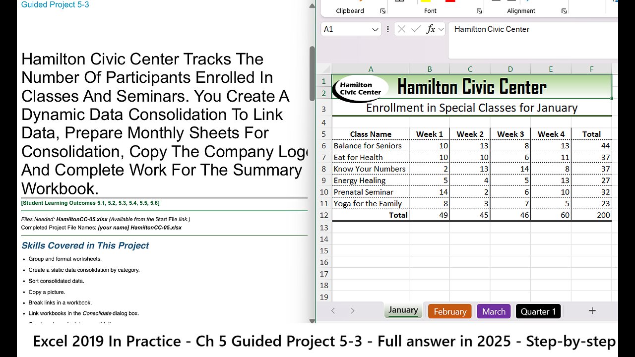
Hamilton Civic Center Tracks The
Number Of Participants Enrolled In
Classes And Seminars. You Create A
Dynamic Data Consolidation To Link
Data, Prepare Monthly Sheets For
Consolidation, Copy The Company Logo,
And Complete Work For The Summary
Workbook.
[Student Learning Outcomes 5.1, 5.2, 5.3, 5.4, 5.5, 5.6]
Files Needed: HamiltonCC-05.xlsx (Available from the Start File link.)
Completed Project File Names: [your name] HamiltonCC-05.xlsx
Skills Covered in This Project
Group and format worksheets.
Create a static data consolidation by category.
Sort consolidated data.
Copy a picture.
Break links in a workbook.
Link workbooks in the Consolidate dialog box.
Create a dynamic data consolidation.
Insert, size, and position a picture.
This image appears when a project instruction has changed to accommodate an update to Microsoft 365
Apps. If the instruction does not match your version of Office, try using the alternate instruction instead.
1/3
https://tulsacc.simnetonline.com/sp/assignments/projects/details/8248556
11/2/23, 5:53 PM Excel 2019 In Practice - Ch 5 Guided Project 5-3 - SIMnet
https://tulsacc.simnetonline.com/sp/assignments/projects/details/8248556 2/3
Figure 5-70 Border tab in Format Cells dialog box
Steps to complete This Project
Mark the steps as checked when you complete them.
1. Open the HamiltonCC-05 start file. The file will be renamed automatically to include your name. Change the project file
name if directed to do so by your instructor, and save it.
NOTE: If group titles are not visible on your Ribbon in Excel for Mac, click the Excel menu and select Preferences to open
the Excel Preferences dialog box. Click the View button and check the Group Titles check box under In Ribbon, Show.
Close the Excel Preferences dialog box.
2. Group the worksheets.
a. Click the January worksheet tab.
b. Press Shift and click the March tab.
3. Format grouped worksheets.
a. Select cells A5:F12.
b. Click the arrow with the Borders button [Home tab, Font group] and select More Borders.
c. Click the Line Color arrow and choose Black, Text 1 (second column).
d. Click the thin solid line Style (bottom choice in the first column of styles).
e. Click the vertical middle of the preview box. If you place a border in the wrong location, click the line in the preview
to remove it.
f. Click the second line Style in the first column (two below None).
g. Click the horizontal middle of the preview box. This border will appear between rows.
h. Click the bottom line Style in the second column (a double border).
i. Click the bottom of the preview area to place a bottom horizontal border (Figure 5-70).
j. Click OK.
4. Enter SUM in grouped worksheets.
a. Select cells F6:F11.
b. Click the Sum button [Home tab, Editing group].
c. Use SUM in cells B12:F12.
d. Click cell A1.
e. Right-click the February sheet tab and choose
Ungroup Sheets.
5. Copy a picture.
a. Click to select the organization logo on the
February sheet.
b. Press Command+C to copy the picture.
c. Click the January sheet tab.
d. Press Command+V to paste the picture.
e. Point to the picture frame to display a move pointer.
f. Drag the picture to fine-tune its location so that it appears in column A to the left of “Hamilton Civic Center.” Nudge
the image with any keyboard directional arrow key. Adjust the width of Column A if necessary.
g. Click cell B1.
6. Copy the March sheet to the end and name it Quarter 1.
7. Set the tab color to Black, Text 1 (second column)
8. Edit cell A3 to read First Quarter Enrollment.
9. Create a static data consolidation by category.
a. Delete the contents of cells A6:E11 on the Quarter 1 sheet. The labels in column A are not in the same order on the
quarterly sheets.
b. Click the Consolidate button [Data tab, Data Tools group].
c. Choose the SUM function.
d. Select and delete references in the All references box.
e. Click the Reference box and click the January tab.
f. Select cells A6:E11 and click + in the Consolidate dialog box.
g. Click the February tab, verify that cells A6:E11 are selected, and click +.
h. Add the March worksheet data to the All references list.
i. Select the Left column box in the Use labels in group (Figure 5-71).
11/2/23, 5:53 PM
Excel 2019 In Practice - Ch 5 Guided Project 5-3 - SIMnet
j. Click OK.
10. Sort consolidated data.
a.
b.
c.
d.
11.
Select cells A6:E11 on the Quarter 1 sheet.
Click the Sort & Filter button [Home tab, Editing
group].
Choose Sort A to Z.
Click cell B1.
Save and close your file (Figure 5-75).
-
 14:47
14:47
GritsGG
1 day agoRumble Tournament Dubular! Rebirth Island Custom Tournament!
62K5 -
 1:36:05
Side Scrollers Podcast
16 hours agoStreamer ATTACKS Men Then Cries Victim + Pronoun Rant Anniversary + More | Side Scrollers
65.6K2 -
 LIVE
LIVE
Lofi Girl
2 years agoSynthwave Radio 🌌 - beats to chill/game to
188 watching -
 42:55
42:55
Stephen Gardner
1 day ago🔥Trump’s SURPRISE Move STUNS Everyone - Democrats PANIC!
83.6K111 -
 1:37:19
Badlands Media
14 hours agoBaseless Conspiracies Ep. 148: The Delphi Murders – Secrets, Setups, and Cover-Ups
33.7K15 -
 5:59:05
SpartakusLIVE
8 hours ago#1 MACHINE Never Stops The GRIND || LAST Stream UNTIL Friday
138K1 -
 28:36
28:36
Afshin Rattansi's Going Underground
1 day agoDoug Bandow: ENORMOUS DAMAGE Done to US’ Reputation Over Gaza, Trump ‘Easily Manipulated’ by Israel
22.6K29 -
 2:45:13
Barry Cunningham
14 hours agoCBS CAUGHT AGAIN! CHICAGO A MESS! LISA COOK IS COOKED AND MORE LABOR DAY NEWS!
102K49 -
 6:39:17
StevieTLIVE
8 hours agoMASSIVE Warzone Wins on Labor Day w/ Spartakus
27.2K1 -
 10:46:42
Rallied
15 hours ago $16.84 earnedWarzone Challenges w/ Doc & Bob
197K4