Excel 2019 In Practice - Ch 5 Guided Project 5-3 - Hamilton Civic Center - Full answer (2025)
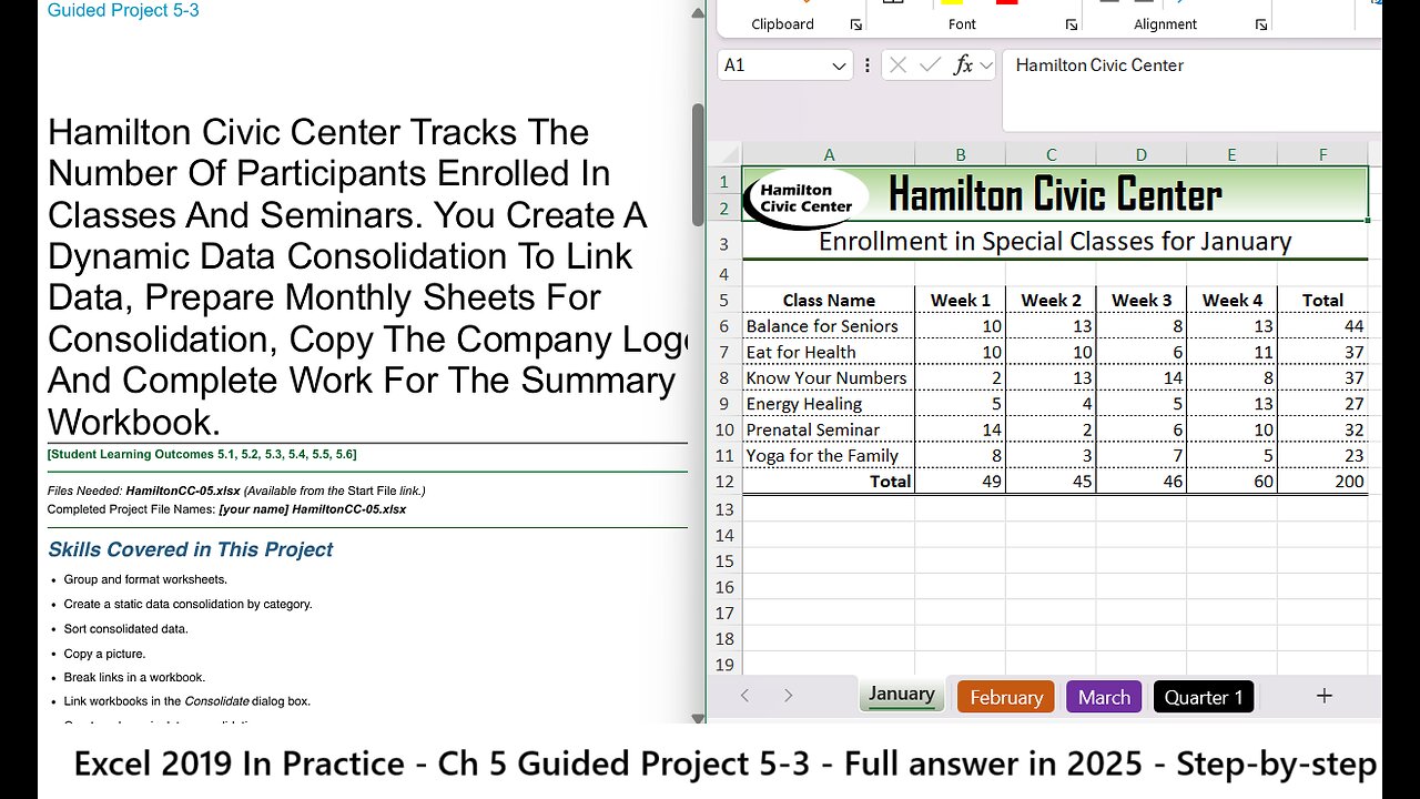
Hamilton Civic Center Tracks The
Number Of Participants Enrolled In
Classes And Seminars. You Create A
Dynamic Data Consolidation To Link
Data, Prepare Monthly Sheets For
Consolidation, Copy The Company Logo,
And Complete Work For The Summary
Workbook.
[Student Learning Outcomes 5.1, 5.2, 5.3, 5.4, 5.5, 5.6]
Files Needed: HamiltonCC-05.xlsx (Available from the Start File link.)
Completed Project File Names: [your name] HamiltonCC-05.xlsx
Skills Covered in This Project
Group and format worksheets.
Create a static data consolidation by category.
Sort consolidated data.
Copy a picture.
Break links in a workbook.
Link workbooks in the Consolidate dialog box.
Create a dynamic data consolidation.
Insert, size, and position a picture.
This image appears when a project instruction has changed to accommodate an update to Microsoft 365
Apps. If the instruction does not match your version of Office, try using the alternate instruction instead.
1/3
https://tulsacc.simnetonline.com/sp/assignments/projects/details/8248556
11/2/23, 5:53 PM Excel 2019 In Practice - Ch 5 Guided Project 5-3 - SIMnet
https://tulsacc.simnetonline.com/sp/assignments/projects/details/8248556 2/3
Figure 5-70 Border tab in Format Cells dialog box
Steps to complete This Project
Mark the steps as checked when you complete them.
1. Open the HamiltonCC-05 start file. The file will be renamed automatically to include your name. Change the project file
name if directed to do so by your instructor, and save it.
NOTE: If group titles are not visible on your Ribbon in Excel for Mac, click the Excel menu and select Preferences to open
the Excel Preferences dialog box. Click the View button and check the Group Titles check box under In Ribbon, Show.
Close the Excel Preferences dialog box.
2. Group the worksheets.
a. Click the January worksheet tab.
b. Press Shift and click the March tab.
3. Format grouped worksheets.
a. Select cells A5:F12.
b. Click the arrow with the Borders button [Home tab, Font group] and select More Borders.
c. Click the Line Color arrow and choose Black, Text 1 (second column).
d. Click the thin solid line Style (bottom choice in the first column of styles).
e. Click the vertical middle of the preview box. If you place a border in the wrong location, click the line in the preview
to remove it.
f. Click the second line Style in the first column (two below None).
g. Click the horizontal middle of the preview box. This border will appear between rows.
h. Click the bottom line Style in the second column (a double border).
i. Click the bottom of the preview area to place a bottom horizontal border (Figure 5-70).
j. Click OK.
4. Enter SUM in grouped worksheets.
a. Select cells F6:F11.
b. Click the Sum button [Home tab, Editing group].
c. Use SUM in cells B12:F12.
d. Click cell A1.
e. Right-click the February sheet tab and choose
Ungroup Sheets.
5. Copy a picture.
a. Click to select the organization logo on the
February sheet.
b. Press Command+C to copy the picture.
c. Click the January sheet tab.
d. Press Command+V to paste the picture.
e. Point to the picture frame to display a move pointer.
f. Drag the picture to fine-tune its location so that it appears in column A to the left of “Hamilton Civic Center.” Nudge
the image with any keyboard directional arrow key. Adjust the width of Column A if necessary.
g. Click cell B1.
6. Copy the March sheet to the end and name it Quarter 1.
7. Set the tab color to Black, Text 1 (second column)
8. Edit cell A3 to read First Quarter Enrollment.
9. Create a static data consolidation by category.
a. Delete the contents of cells A6:E11 on the Quarter 1 sheet. The labels in column A are not in the same order on the
quarterly sheets.
b. Click the Consolidate button [Data tab, Data Tools group].
c. Choose the SUM function.
d. Select and delete references in the All references box.
e. Click the Reference box and click the January tab.
f. Select cells A6:E11 and click + in the Consolidate dialog box.
g. Click the February tab, verify that cells A6:E11 are selected, and click +.
h. Add the March worksheet data to the All references list.
i. Select the Left column box in the Use labels in group (Figure 5-71).
11/2/23, 5:53 PM
Excel 2019 In Practice - Ch 5 Guided Project 5-3 - SIMnet
j. Click OK.
10. Sort consolidated data.
a.
b.
c.
d.
11.
Select cells A6:E11 on the Quarter 1 sheet.
Click the Sort & Filter button [Home tab, Editing
group].
Choose Sort A to Z.
Click cell B1.
Save and close your file (Figure 5-75).
-
 2:19:30
Side Scrollers Podcast
18 hours agoAngry Joe’s TDS/Halo Meltdown + Console War is OVER + Twitch Staff FIRED + More | Side Scrollers
65.9K15 -
 19:23
19:23
Nikko Ortiz
2 days agoRealistic Halloween Horror Movie Deaths
24.5K11 -
 18:09
18:09
The Pascal Show
9 hours ago $2.24 earnedHE'S PANICKING?! FBI Director Kash Patel Shuts Down Investigation Into Charlie Kirk Assassination
3.56K12 -
 34:55
34:55
BlabberingCollector
1 day agoHBO Set Leaks, Audible AudioBooks Paves New Harry Potter Future, & More! | Wizarding World Roundup
6.25K3 -
 LIVE
LIVE
Lofi Girl
3 years agolofi hip hop radio 📚 - beats to relax/study to
118 watching -
 25:03
25:03
GritsGG
14 hours agoHow to Obtain Warzone VICTORY From a TREE! Casual Solo Gameplay!
14.9K4 -
 2:48:05
FreshandFit
10 hours agoGhetto Fake Russian Disrespected The Entire Panel & THIS Happened...
244K156 -
 1:27:57
Tucker Carlson
7 hours agoTucker and Col. MacGregor Warn How Neocons Are Exploiting the Drug Crisis to Drag America Into War
39.3K150 -
 2:08:50
Badlands Media
12 hours agoDevolution Power Hour Ep. 402: Arctic Frost, Trump’s Third Term & The G2 Showdown
92.7K56 -
 2:05:48
Inverted World Live
10 hours agoUFO Seen Over Tokyo During Trump Visit | Ep. 132
69.5K21