Excel 2019 In Practice - Chapter 3 Guided Project 3-3 - Blue Lake Sports - Update 2025

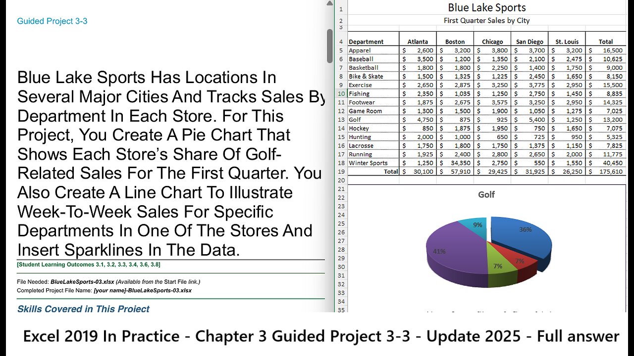
Blue Lake Sports Has Locations In
Several Major Cities And Tracks Sales By
Department In Each Store. For This
Project, You Create A Pie Chart That
Shows Each Store’s Share Of Golf
Related Sales For The First Quarter. You
Also Create A Line Chart To Illustrate
Week-To-Week Sales For Specific
Departments In One Of The Stores And
Insert Sparklines In The Data.
[Student Learning Outcomes 3.1, 3.2, 3.3, 3.4, 3.6, 3.8]
File Needed: BlueLakeSports-03.xlsx (Available from the Start File link.)
Completed Project File Name: [your name]-BlueLakeSports-03.xlsx
Skills Covered in This Project
Create, size, and position a pie chart object.
Apply a chart style.
Change the chart type.
Add and format chart elements.
Create a line chart sheet.
Apply a chart layout.
Insert and format sparklines in a worksheet.
This image appears when a project instruction has changed to accommodate an update to Microsoft 365
Apps. If the instruction does not match your version of Office, try using the alternate instruction instead.
1/5
https://tulsacc.simnetonline.com/sp/assignments/projects/details/8248554
10/28/23, 5:55 PM Excel 2019 In Practice - Ch 3 Guided Project 3-3 - SIMnet
https://tulsacc.simnetonline.com/sp/assignments/projects/details/8248554 2/5
Steps to complete This Project
Mark the steps as checked when you complete them.
1. Open the BlueLakeSports-03 start file. If the workbook opens in Protected View, click the Enable Editing button so
you can modify it. The file will be renamed automatically to include your name. Change the project file name if directed to
do so by your instructor, and save it.
NOTE: If group titles are not visible on your Ribbon in Excel for Mac, click the Excel menu and select Preferences to open
the Excel Preferences dialog box. Click the View button and check the Group Titles check box under In Ribbon, Show.
Close the Excel Preferences dialog box.
2. Create a pie chart object.
a. Select the Revenue by Department sheet, select cells A4:F4, press command, and select cells A13:F13.
b. Click the Recommended Charts button [Insert tab, Charts group].
c. Choose Pie.
3. Apply a chart style.
a. Select the chart object.
b. Click the More button [Chart Design tab, Chart Styles group].
c. Select Style 12.
4. Size and position a chart object.
a. Point to the chart object border to display the move pointer.
b. Drag the chart object so its top-left corner is at cell A21.
c. Point to the bottom right selection handle to display the resize arrow.
d. Drag the pointer to cell G36.
5. Change the chart type.
a. Select the pie chart object and click the Change Chart Type button [Chart Design tab, Type group].
b. In the drop-down list point to Pie.
c. Choose 3-D Pie