New Perspectives Excel 2019 | Module 4: End of Module Project 1 | FLO Biotech (Update 2025)

FLO Biotech
ANALYZE AND CHART FINANCIAL DATA

GETTING STARTED
• Open the file NP_EX19_EOM4-1_FirstLastName_1.xlsx, available for download from the SAM website.
• Save the file as NP_EX19_EOM4-1_FirstLastName_2.xlsx by changing the “1” to a “2”.
o If you do not see the .xlsx file extension in the Save As dialog box, do not type it. The program will add the file extension for you automatically.
• With the file NP_EX19_EOM4-1_FirstLastName_2.xlsx still open, ensure that your first and last name is displayed in cell B6 of the Documentation sheet.
o If cell B6 does not display your name, delete the file and download a new copy from the SAM website.
PROJECT STEPS
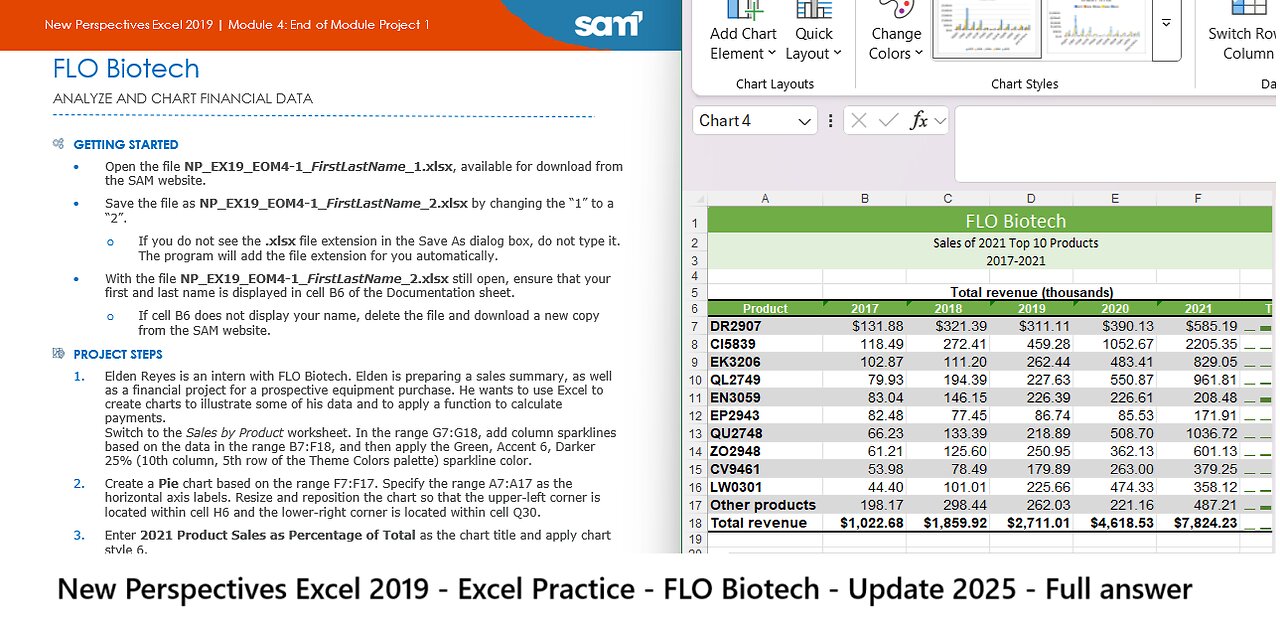
1. Elden Reyes is an intern with FLO Biotech. Elden is preparing a sales summary, as well as a financial project for a prospective equipment purchase. He wants to use Excel to create charts to illustrate some of his data and to apply a function to calculate payments.
Switch to the Sales by Product worksheet. In the range G7:G18, add column sparklines based on the data in the range B7:F18, and then apply the Green, Accent 6, Darker 25% (10th column, 5th row of the Theme Colors palette) sparkline color.
2. Create a Pie chart based on the range F7:F17. Specify the range A7:A17 as the horizontal axis labels. Resize and reposition the chart so that the upper-left corner is located within cell H6 and the lower-right corner is located within cell Q30.
3. Enter 2021 Product Sales as Percentage of Total as the chart title and apply chart style 6.
4. Create a 2-D Line chart based on the range B18:F18. Modify the chart by changing the horizontal axis labels to use the range B6:F6. Enter Total Revenue by Year (Millions) as the chart title, and resize and reposition the chart so that the upper-left corner is located within cell A20 and the lower-right corner is located within cell G37.
5. Apply chart style 13 to the line chart you just created. Format the vertical axis to use a maximum value of 8000, change Display units to Thousands but don't show the units on the chart, and show 0 decimal places in the axis labels.
6. Create a stacked column chart based on the range A6:F17. Modify the chart by switching the row and column so the horizontal axis shows years and the stacked components of each bar are products. Enter Product Contribution to Total Revenue 2017-2021 (millions) as the chart title, and resize and reposition the chart so that the upper-left corner is located within cell A38 and the lower-right corner is located within cell G63.
7. Apply chart style 9 to the stacked column chart you just created. Format the vertical axis to use a maximum value of 8000, change Display units to Thousands but don't show the units on the chart, and show 0 decimal places in the axis labels.
8. Create a 3-D Clustered Column chart based on the range A6:F17. Resize and reposition the chart so that the upper-left corner is located within cell H32 and the lower-right corner is located within cell Q52. Remove the 2018, 2019, and 2020 series from the legend and chart area.
9. Enter 2017 and 2021 Revenue Comparison by Product as the chart title and then format the chart title as 16 point bold text. Enter Total revenue (thousands) as the vertical axis title.
10. Change the background color of the plot area to White, Background 1 and then change the background color of the chart area to Green, Accent 6, Lighter 80% (10th column, 2nd row in the Theme Colors palette).
Your workbook should look like the Final Figures on the following pages. Save your changes, close the workbook, and then exit Excel. Follow the directions on the SAM website to submit your completed project.
 
Final Figure 1: Sales by Product Worksheet