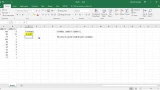
How to find Correlation Coefficient in Excel? | Excel Training | Statistics
#Excel #statistics #correlation
The correlation coefficient is a statistical measure that describes the strength and direction of the linear relationship between two variables. It ranges from -1 to 1, where -1 indicates a perfect negative linear relationship, 0 indicates no linear relationship, and 1 indicates a perfect positive linear relationship. The closer the correlation coefficient is to 1 or -1, the stronger the relationship between the variables.
Finding the Correlation Coefficient in Excel:
To find the correlation coefficient in Excel, you can use the "CORREL" function. The syntax for the function is as follows:
=CORREL(array1, array2)
Where "array1" and "array2" are the ranges of cells that contain the data sets that you want to compare. The function will return a value between -1 and 1, where -1 indicates a perfect negative correlation, 0 indicates no correlation, and 1 indicates a perfect positive correlation.
For example, if you have data in cells A1:A10 and B1:B10, you can use the following formula to find the correlation coefficient:
=CORREL(A1:A10, B1:B10)
Note: If you are using an older version of Excel (2003 and earlier) you may need to use a different function, like PEARSON.
Using Data Analysis
We can also analyze the given dataset and calculate the correlation coefficient: To do so follow the below steps:
Step 1: First you need to enable Data Analysis ToolPak in Excel. To enable :
Go to File tab in the top left corner of the Excel window and choose Options.
The Excel Options dialog box opens. Now go to the Add-Ins option and in the Manage select Excel Add-ins from the drop down.
Click on Go button.
The Add-ins dialog box opens. In this check the option Analysis ToolPak.
Click OK!
Step 2: Now click on Data followed by Data Analysis. A dialog box will appear.
Step 3: In the dialog box select Correlation from the list of options. Click OK!
Step 4: The Correlation menu will appear.
Step 5: In this menu first provide the Input Range. The input range is the cell range of X and Y.
Step 6: Also, supply the Output Range as the cell number where you want to display the result. By default, the output will appear in the new Excel sheet in case if you don’t provide any Output Range.
Step 7: Check the Labels in first-row option if you have labels in the dataset.
Step 8: Click OK.
Step 9: The Data Analysis table is now ready. Here, you can see the correlation coefficient between X and Y.
-
 0:45
0:45
Performing in an Academic Environment
3 years agoMicrosoft Excel Tutorial - Correlation
89 -
 8:38
8:38
AccountingInstruction
8 months agoCorrelation Simple Few Data Points Example 1 Statistics & Excel
-
 8:08
8:08
AccountingInstruction
8 months agoStatistics & Excel Correlation Simple Few Data Points Example 2
-
 5:09
5:09
AccountingInstruction
8 months agoCorrelation Calculation with Strange Result 1 Statistics & Excel
-
 4:50
4:50
AccountingInstruction
8 months agoCorrelation Calculation with Strange Result 2 Statistics & Excel
-
 0:58
0:58
AccountingInstruction
8 months agoStatistics & Excel Perfect Positive Correlation
-
 20:59
20:59
AccountingInstruction
8 months agoCorrelation Large Data Sets Focus of Z Score Relationship Part 1 1750 Statistics & Excel
1 -
 22:41
22:41
AccountingInstruction
8 months agoCorrelation Random Number Generation Example Part 2 1732 Statistics & Excel
-
 0:58
0:58
AccountingInstruction
9 months agoStatistics & Excel Height Statistical Inference Data - Excel Practice Problem
-
 4:58
4:58
AccountingInstruction
8 months agoPerfect Positive Correlation Part 4 Statistics & Excel